How To Change Case in Microsoft Excel Tutorial

Introduction To Using Change Case in Microsoft Excel

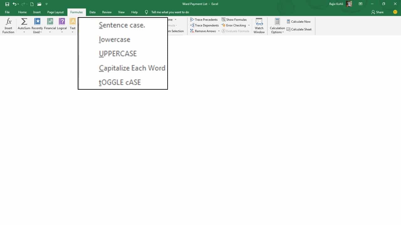
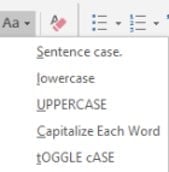
Truly, I missed a few points in the Change Case in Microsoft Excel Video tutorial, which I will briefly explain here. If you are familiar with Microsoft Word then you might know that it is easy to Change Case of Text in 5 different formats: Sentence case, lower case, UPPER CASE, Capitalize Each Word and tOGGLE cASE. You may always want to have the “Change Case” command in Microsoft Excel as well but unfortunately, this magic button is not available in Excel and you need to use Functions to accomplish the same task which is easy to use even for beginners.

For instance, here we have a list of a few people with Sr No., Name, Total Population Surveyed, Total Days Worked, Rate Days, and Amount (see Figure 1.1). We need to change the case of the Name field to UPPER CASE. To do this, we can use Microsoft Excel functions but they are limited to only 3 Change Case styles: Upper, Lower, and Proper Case (Proper is called Sentence case in Word). All these functions are related to the Text Function Category of Excel.

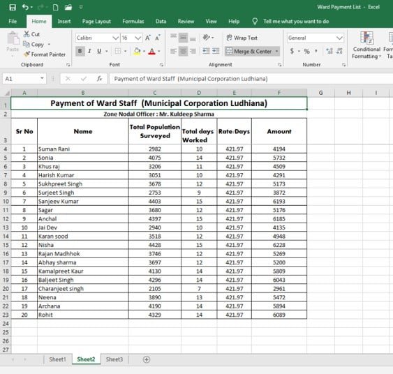
Sample Worksheet For Change Case in Microsoft Excel — Name Begins from Cell Reference B4 (B Column for Names and first record “Suman Rani” begins at Row Number 4)
Figure 1.1

You can either use the very next empty column in the list to type one of the 3 functions, which in our case is Column G or you can insert a New Column between Column B and C. Use the last column to write the function or insert a new column between; are two separate methods of changing text case in Microsoft Excel.

Using The Last Column to Change the Case of Text

So let’s first use Column G to type our function to change all the names in the list to UPPER case. In Cell G4 type :

=UPPER(B4)

B4 Cell Reference as the list of Names is in Column B and starting from the 4th row and then Press Enter Key. Now, we need to copy the same formula to the rest of the cells below in Column G up to Row 23 because it will convert only one record value from Cell B4 into G4. We will copy the above formula up to Row Number G23 because our name list ends at B23. See Figure 1.2:

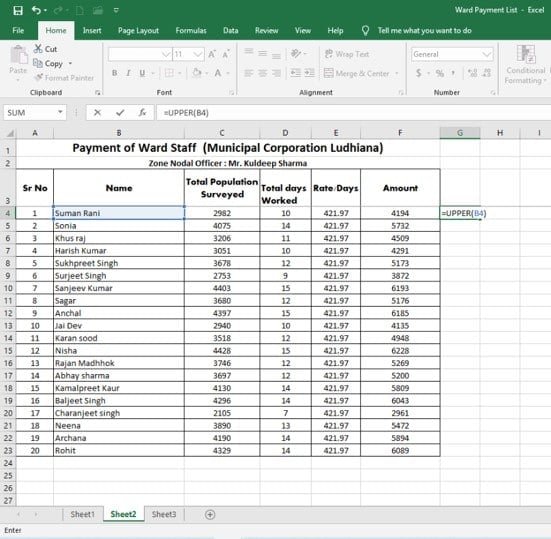
Upper Function in Microsoft Excel — Typing Upper function in Cell G4 and giving the reference of Cell B4 within Parenthesis for Text value i.e. our Cell Reference. Pressing the Enter key will convert the value of Cell B4 which is Suman Rani – as SUMAN RANI in uppercase in Cell G4.
Figure 1.2

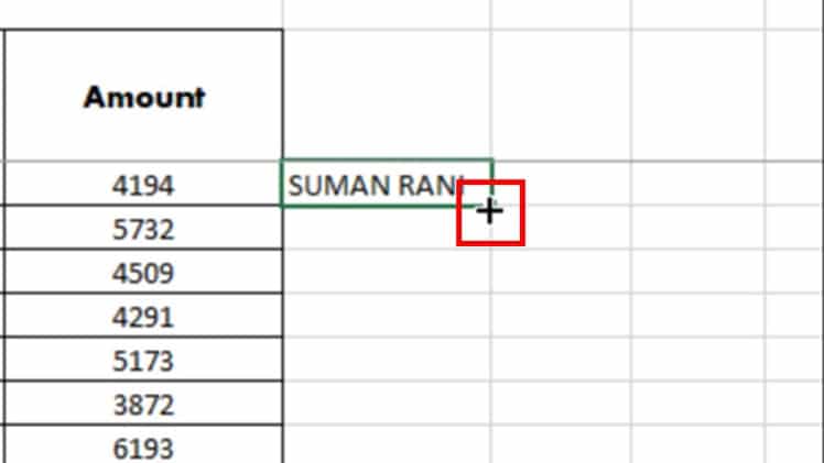
There are various ways in Excel to copy formulas and you can use the traditional method of using Copy and Paste command or you can double-click the Black Square icon in the corner of cell G4 as shown having a Cross Mouse Pointer when the mouse hovered over it. See Figure 1.3:

Cross Mouse Pointer in Excel during Copying — A Cross Appears when you hover your pointer over Black Rectangle in Microsoft Excel
Figure 1.3

Now, you can either drag-n-drop the Cross Mouse Pointer up to G23 or you can double-click on the Black Rectangle, and that way it will AutoFill the formula to the rest of the cells up to G23. See Figure 1.4:

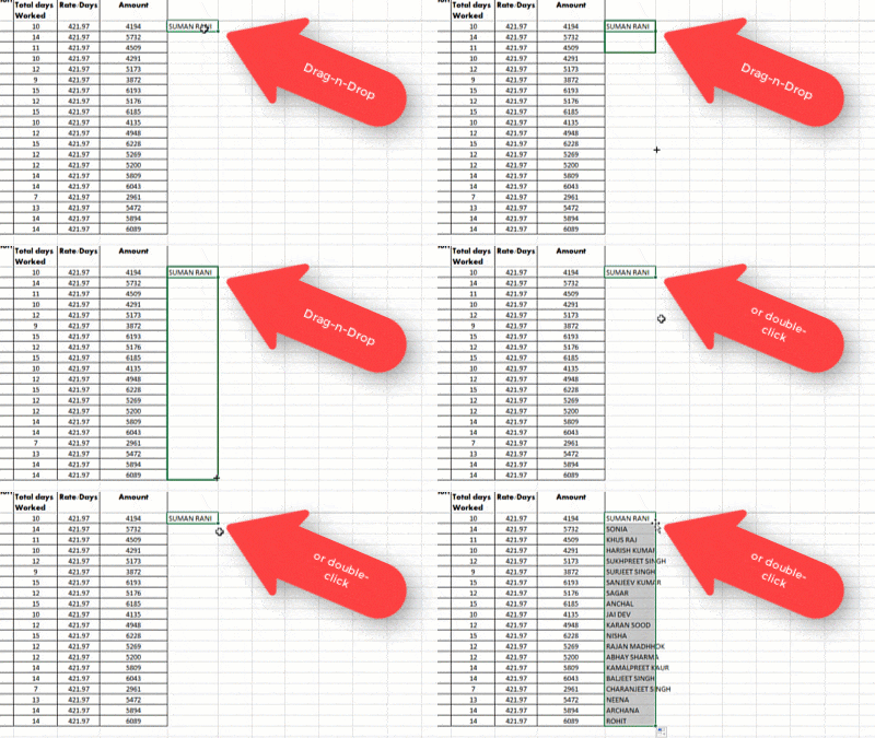
How To Copy Formulas in Microsoft Excel — Two ways of copying formulas (or you can also call it Auto Fill cells)
Drag and Drop or Double-click on Black Rectangle at bottom right corner of the cell
Figure 1.4

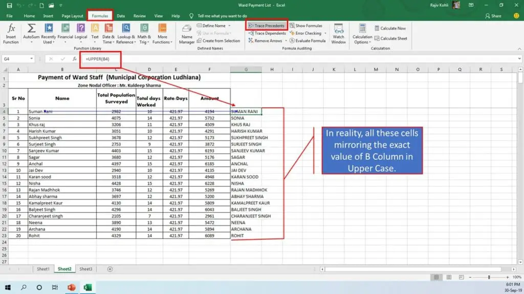
But we need these values in B4 to B23 cells with the changed case to Upper. But first, take a look at Figure 1.5:

Upper Case Function in Excel — You just cannot simply Cut or Copy these values from Column G to Column B.
Figure 1.5

As shown in Figure 1.5 the values in Column G are not actual values but they are mirrored values of Column B in Upper Case and in-reality all these Cells contain formulas and in Excel, you can’t just Copy / Cut and Paste these values and replace them with the original. It means you are going to remove the original values from which your Upper() function was fetching the data.
The formula bar shows the exact value of Cell G4, which is “=Upper(B4)” not SUMAN RANI in Upper Case. The Trace Precedents command from the Formulas tab indicates that the value in Cell G4 depends on the value of Cell B4. So, if you will replace the original value of B4 with G4 then now from which cell the formula will fetch the values? You can see the results shown in Figure 1.6:

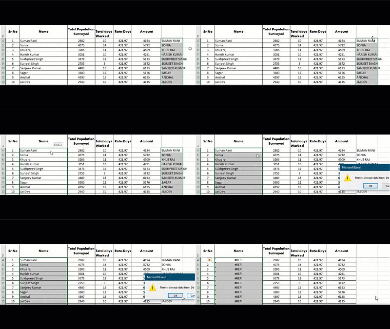
Replacing Contents With Formulas in Excel — #Ref error displays when a formula references a cell which is no longer exists.
Figure 1.6

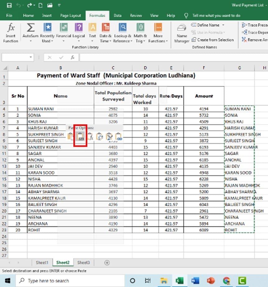
So here is the right way to replace the values of cell references B4:B23 with cell references G2:G23. Select Cells from G2 to G23 and then either press CTRL+C for Copy or Right-Click and then choose Copy from the Context menu. You will start seeing a dashed border around the copied cells. See Figure 1.7:

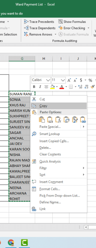
How to Copy in Microsoft Excel — Click to Enlarge
The dotted border indicates that values have been Copied to the clipboard after clicking on Copy from the context menu
Figure 1.7

The last step is to right-click on Cell B4 and from under Paste Options press the 2nd button showing a ToolTip as Values. This Paste as Values will now replace all the original values from B4 to B23 with the values (not formulas this time) that Microsoft Excel getting with the Upper() function on G Column. See Figure 1.8:

You cannot use Cut command because you will then not see Paste as Values option in right-click Context menu.

Paste As Value in Microsoft Excel — Click to Enlarge. Figure 1.8
Copied from G4:G23 and Pasted as Values on B4:B23

You will immediately start seeing a Live Preview in the background when you will hover your mouse over the Paste as Values option. Later, you can delete the formulas from cells G4 to G23 as we no longer need them. If you want the output in any of the other 2 Text Case Styles, like:
- use =lower(text) – to convert all to lowercase text
- use =proper(text) – To Convert All To Title Case

Where (text) is the reference of the cell whose value you want in that particular text case e.g. =lower(b4)

Second Method of Inserting a Column Between

This method is just a replication of the above method but the only difference is that you are not using the last column for Upper(), Lower(), or Proper() functions instead you will first:

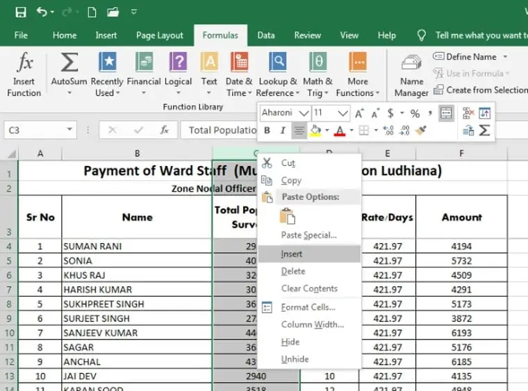
Insert a New Column between Columns B and C by right-clicking on Column C and then choosing Insert from the context menu. See Figure 1.9:

How to Insert a Column in Excel — Right-Click on Column C and choose Insert from Context menu
Figure 1.9

Then you will need to repeat all the steps mentioned above from Figure 1.2 to Figure 1.8 but this time replace the values of B4:B23 with C4:C23.
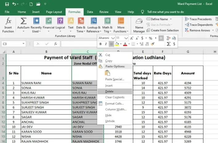
Also adding a further step of deleting the newly inserted Column C after Pasting as Values on Column B. See Figure 1.10:

How To Delete A Column in Microsoft Excel

The only difference in the above two methods is which column you choose to type the formula, that’s it! You can use any column to enter the change text case formula and of course, you can make a guess which one of the above methods is much easier. There is one more method, which is taking the help of Microsoft Word to Change the Case of Text in Excel. Watch our video to learn more.

I hope you got The Teacher Point.